SCENARIO
You are a junior data analyst working in the marketing analyst team at Cyclistic, a bike-share company in Chicago. The director of marketing believes the company’s future success depends on maximizing the number of annual member riderships. Therefore, your team wants to understand how casual riders and annual member riders use Cyclistic bikes dierently. From these insights, your team will design a new marketing strategy to convert casual riders into annual member riders.
But first, Cyclistic executives must approve your recommendations, so they must be backed up with compelling data insights and professional data visualizations.
CHARACTERS AND TEAM
- Cyclistic: A bike-share program that features more than 5,800 bicycles and 600 docking stations. Cyclistic sets itself apart by also oering reclining bikes, hand tricycles, and cargo bikes, making bike-share more inclusive to people with disabilities and riders who can’t use a standard two-wheeled bike. The majority of riders opt for traditional bikes; about 8% of riders use the assistive options. Cyclistic riders are more likely to ride for leisure, but about 30% use them to commute to work each day.
- Lily Moreno: The director of marketing and your manager. Moreno is responsible for the development of campaigns and initiatives to promote the bike-share program. These may include email, social media, and other channels.
- Cyclistic marketing analytics team: A team of data analysts who are responsible for collecting, analyzing, and reporting data that helps guide Cyclistic marketing strategy. You joined this team six months ago and have been busy learning about Cyclistic’s mission and business goals — as well as how you, as a junior data analyst, can help Cyclistic achieve them.
- Cyclistic executive team: The notoriously detail-oriented executive team will decide whether to approve the recommended marketing program.
ABOUT COMPANY
In 2016, Cyclistic launched a successful bike-share offering. Since then, the program has grown to a fleet of 5,824 bicycles that are geotracked and locked into a network of 692 stations across Chicago. The bikes can be unlocked from one station and returned to any other station in the system anytime.Until now, Cyclistic’s marketing strategy relied on building general awareness and appealing to broad consumer segments. One approach that helped make these things possible was the flexibility of its pricing plans: single-ride passes, full-day passes, and annual member riderships. Customers who purchase single-ride or full-day passes are referred to as casual riders. Customers who purchase annual member riderships are Cyclistic member riders.
Cyclistic’s finance analysts have concluded that annual member riders are much more profitable than casual riders. Although the pricing flexibility helps Cyclistic attract more customers, Moreno believes that maximizing the number of annual member riders will be key to future growth. Rather than creating a marketing campaign that targets all-new customers, Moreno believes there is a very good chance to convert casual riders into member riders. She notes that casual riders are already aware of the Cyclistic program and have chosen Cyclistic for their mobility needs.
Moreno has set a clear goal: Design marketing strategies aimed at converting casual riders into annual member riders. In order to do that, however, the marketing analyst team needs to better understand how annual member riders and casual riders differ, why casual riders would buy a member ridership, and how digital media could affect their marketing tactics. Moreno and her team are interested in analyzing the Cyclistic historical bike trip data to identify trends.
Lily Moreno (Marketing Director and Manager) asked us to answer the first question: "How do annual member riders and casual riders use Cyclistic bikes differently?".
For reminder, Moreno's interest was clear: "Moreno and her team are interested in analyzing the Cyclistic historical bike trip data to identify trends."
| Study Case Roadmap - Ask |
|---|
| Guidance Question: |
| Key Tasks: |
| Result |
I must first download the data from here before beginning the analysis. The data was stored as a .csv file within the .zip archive. All files were separated by month using the naming format 'yyyymm_datasetname'. The stakeholders requested that we analyze the 12-month data. This analysis was initiated on October 18th 2022, thus the most recent available complete data was from September 2022. I therefore downloaded data from October 2021 to September 2022.
This data is publicly accessible under the terms of the license found here, which states that personal information such as riders' names, addresses, genders, and credit card numbers are not included. All downloaded information was saved to the local computer.
To prevent data management errors, I created a folder hierarchy to store the data. Inside the "cyclistic" main folder, I created the "data prepare" folder to store all downloaded data. To conduct a preliminary analysis, I opened all the data and looked for inconsistencies. There was an inconsistency in the ride_id data despite the fact that the data had the same structure (13 columns) and names.
All columns name: ride_id, rideable_type, started_at, ended_at, start_station_name, start_station_id, end_station_name, end_station_id, start_lat, start_lng, end_lat, end_lng, member_casual.
In this version of analysis, I used Microsoft Excel, MySQL Workbench, and Microsoft Power BI as analysis tools, along with MySQL and DAX as programming languages.
| Study Case Roadmap - Prepare |
|---|
Guidance Question:
|
Key Tasks:
|
Microsoft Excel was primarily used to clean the data, whereas MySQL Workbench was used to build a database and perform advance data cleaning.
As previously stated, there were irregularities in ride_id data. The ride_id column has variable character data type, which includes both characters and numbers, however the wrong data has a numeric data type with a large exponential. To resolve this issue, I use this function to determine how many characters are in the correct ride data:
=LEN([ride_id cell])
=16
Once the results has been known, I must extract 16 characters from the wrong data. Due to a large exponential, the wrong data contain many zeros, hence I must use this method to extract all values before the zeros:
=LEFT([ride_id cell], 16)
There are numbers with three trailing zeros and numbers with two trailing zeros. To correct this, I used the letter 'Z' as the leading character, 'Z' as the trailing character for the number with two trailing zeros, and 'ZZ' as the trailing character for the number with three trailing zeros. Since the letter 'Z' has never appeared in the data, I use it as a mark, too. I used the following function:
# two trailing zeros number: '9984119508987300'
=CONCATENATE("Z", LEFT([ride_id cell], 14), "Z")
=Z99841195089873Z

# three trailing zeros number: '9841195089873000'
=CONCATENATE("Z", LEFT([ride_id cell], 13), "ZZ")
=Z9841195089873ZZ
After correcting the ride id data, I continued to check each data type, resulting in the following:
| Column Name | Data Type |
|---|---|
| ride_id | text/variable characters |
| rideable_type | text |
| started_at | datetime (format: mm/dd/yyyy hh:mm:ss AM/PM) |
| ended_at | datetime (format: mm/dd/yyyy hh:mm:ss AM/PM) |
| start_station_name | text/variable characters |
| start_station_id | text/variable charactes |
| end_station_name | text/variable charactes |
| end_station_id | text/variable charactes |
| start_lat | decimal number |
| start_lng | decimal number |
| end_lat | decimal number |
| end_lng | decimal number |
| member_casual | text |
The date format differs from MySQL's format, which is 'yyyy-mm-dd hh:mm:ss.' I will handle this using SQL script. There were also blank station names and station id, which I will also replace using SQL script due to the huge data volume (>5 million rows) that Excel cannot handle.
All cleaned data were stored in a new folder titled 'data clean' with the file name format 'Cyyyymm-dataname.csv', where the letter 'C' signifies cleansed.
I created a schema (database) named 'cyclistic' in MySQL Workbench and used the following script to create a table for each data:
/*Activate the schema*/
USE cyclistic;

/*Create table with the table naming format 'td_yymm' with td means trip data*/
CREATE TABLE td_yymm (
	ride_id TEXT,
    rideable_type TEXT,
    started_at DATETIME,
    ended_at DATETIME,
    start_station_name TEXT,
    start_station_id TEXT,
    end_station_name TEXT,
    end_station_id TEXT,
    start_lat DOUBLE,
    start_lng DOUBLE,
    end_lat DOUBLE,
    end_lng DOUBLE,
    member_casual TEXT
    );

/*Load data into the table*/
LOAD DATA LOCAL
	INFILE '\\data_clean\\Cyyyymm-tripdata.csv'
    INTO TABLE cyclistic.td_yymm
    FIELDS TERMINATED BY ','
    ENCLOSED BY '"'
    LINES TERMINATED BY '\n'
    IGNORE 1 ROWS;
    (
    column_1, @column_date, column_3
    )
    SET columnn_date_name = str_to_date(@column_date_name, '%m/%d/%Y %r')

    /* this line convert the date format from mm/dd/yyyy hh:mm:ss AM/PM to the
    standard datetime format in MySQL (yyyy-mm-dd hh:mm:ss), the %r means the
    time format hh:mm:ss AM/PM in 12-hour format */
Next step, I need to combine all table into one using this script:
/*Create a new table - copy the table schema using LIKE operator */
create table td_all like td_yymm;

/*Insert the data from all table using UNION ALL operator*/
INSERT INTO cyclistic.td_all (column_1,
									column_2,
									column_3,
                                    ...
									)
SELECT * FROM cyclistic.td_2209
UNION ALL
...
UNION ALL
SELECT * FROM cyclistic.td_2110
;
Now, I can continue to advance data cleaning.
The first thing I did was check for duplication using the following script:
SELECT
    COUNT(ride_id) - COUNT(DISTINCT ride_id) as duplicate
FROM cyclistic.td_all;

/* Result, duplicate = 0 */
This script computes the difference between the total number of ride_id rows and the number of unique ride_id rows, with the remainder equaling the number of duplicates. As a result, there were no duplicates among the data. Using the given latitude and longitude data, I must then fill the blank field in station name and id. Using this script, I had to create an index for known and blank station name & id.
SELECT *
FROM cyclistic.td_all
WHERE start_lat in
			(SELECT
				start_lat
			FROM cyclistic.td_all
			WHERE start_station_name = ""
			GROUP BY 1)
    AND start_lng in
			(SELECT
				start_lng
			FROM cyclistic.td_all
			WHERE start_station_name = ""
			GROUP BY 1)
GROUP BY start_lat, start_lng
ORDER BY start_lat, start_lng DESC
;
This script selects all data with latitude and longitude equal to the blank field, resulting in a table including both known and blank station names and id. Then, I exported this table to the "data clean" folder with the filename "td_all_index.csv". I then open the index file in Microsoft Excel, create a duplicate table, and use the INDEX MATCH formula to fill in the blanks.
# 1. How to find the blank station name
=INDEX([station_name_range], MATCH(1, ([lat_1]=[lat_range])*([lng_1]=[lng_range]), 0))

# 1.1 implementation
=INDEX($C$2:$C$627, MATCH(1,(N2=$G$2:$G$627)*(O2=$H$2:$H$627),0))
EXPLANATION: The INDEX() function requires at least two parameters: an array/reference and a row number. The [station_name_range] is the reference, so I must lock the range with the $ sign, and the MATCH() function will identify the row number that meets the criteria (exact same latitude and longitude). The MATCH() function requires two parameters and a type of match. The first piece of information is the desired value, followed by the lookup array. The lookup array consisted of the result of a logical operation, which stated that if the lat_1 matches with the lat_range, it equals TRUE, and if the lng_1 matches with the lng_range, it equals TRUE, then TRUE multiplied by TRUE equals 1 (TRUE AND TRUE = TRUE), so the criteria is extremely strict. The value 0 in the match type field indicates that I want to search for the precise value, which was 1.
# 2.1 How to find the blank station id
=INDEX([station_id_range], MATCH(TRUE,([station_name_1]=[station_name_range]),0))

# 2.2 Implementation
=INDEX($D$2:$D$627, MATCH(TRUE,([@[start_station_name]]=$C$2:$C$627),0))
EXPLANATION: This formula is actually the same, but I just used the boolean value to look the exact same station id from the station name.
Then, I update the table in MySQL Workbench using this script:
/* This script also used for the end station name and id */
UPDATE cyclistic.td_all
SET start_station_name = CASE
		WHEN start_lat = [latitude_1] AND start_lng = -[longitude_1] THEN start_station_name = '[station_name_1]'
		...
		WHEN start_lat = [latitude_n] AND start_lng = -[longitude_n] THEN start_station_name = '[station_name_n]'
        ELSE start_station_name END
        ,
	start_station_id = CASE
		WHEN start_station_name = '[station_name_1]' THEN start_station_id = '[id_1]'
		...
		WHEN start_station_name = '[station_name_n]' THEN start_station_id = '[id_n]'
		ELSE start_station_id END
WHERE start_station_name = "";
EXPLANATION: I utilize the CASE WHEN statement to automatically insert particular values (after THEN statement) that meet a specific condition (after WHEN statement) into each of the hundreds of blank fields. Additionally, I must filter the query with the WHERE clause so that it affects only the blank data field; otherwise, it will effect the entire dataset.
Finally, the data that hadn't matched to any latitude and longitude will be filled with "unknown" using this script:
/* Also use this script for the end station name */
UPDATE cyclistic.td_all
SET start_station_name = 'unknown'
WHERE start_station_name = "";

/* Check if there is any blank field left*/
SELECT * FROM cyclistic.td_all WHERE start_station_name = "";
/* Result = 0 - All blanks has been replace by unknown*/
Before proceeding to the analysis process, I want to ensure that there is no duplication, so I rerun the duplication check script, which returned 1.3 million duplicate rows of data. I resolved the issue using the following script:
/* Make a temp table */
CREATE TABLE cyclistic.td_all_temp LIKE cyclistic.td_all;

/* Insert all data in the previous
table into the temp table using SELECT DISTINCT statement*/
INSERT INTO cyclistic.td_all_temp
SELECT DISTINCT * FROM cyclistic.td_all;

/* TRUNCATE and DROP the previous table.
Truncate is mandatory to reclaim local disk space*/
TRUNCATE TABLE cyclistic.td_all;
DROP TABLE cyclistic.td_all;

/* Rename the temp table to previous table name*/
ALTER TABLE cyclistic.td_all_temp rename to td_all;
Now the table is ready to be analyzed.
| Case Study Roadmap - Process |
|---|
Guiding questions:
|
Key tasks:
|
Tools I used to analyze are mainly Power BI and not predominantly MySQL Workbench.
Raw data could not yet be analyzed; therefore, I was required to remove or aggregate the data before proceeding with further analysis. First, I created a SQL script in MySQL Workbench to extract the day and month from the datetime data and to aggregate the ride duration in minutes. This script executes the day and month name extraction:
/* Duration is in SECOND*/
SELECT
    *,
    dayname(started_at) as day_name,
    monthname(started_at) as month_name,
    timestampdiff(second, started_at, ended_at) as duration
FROM
    cyclistic.td_all
ORDER BY
    timestampdiff(second, started_at, ended_at) ASC;
EXPLANATION: dayname() and monthname() functions extracted the name of the day and month from the selected date data. timestampdiff() function automatically aggregated value by substracting the start and end datetime. This function can convert the time unit from microseconds to year, but I used second as the time unit to see more detail data.
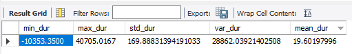
As a result, approximately 130,000 rows of data had ride duration equal to zero seconds. It could be an error, a bike docking, or a ride cancellation. Therefore, I used this SQL script to summarize the table to determine if there were any issues:
/* I made an temporary table using the WITH statement
to do data exploration, duration is in MINUTE */
WITH td_c as (
			SELECT
				*,
				dayname(started_at) as day_start,
				timestampdiff(second, started_at, ended_at)/60 as duration
			FROM
				cyclistic.td_all
                )
/* In this SELECT statement, I made a summary table
to see data distribution */
SELECT
    min(duration) as min_dur,
    max(duration) as max_dur,
    stddev(duration) as std_dur,
    variance(duration) as var_dur,
    avg(duration) as mean_dur
FROM
	td_c
The result is:
/* I used the same temp table, then filtered it to only view the data with duration below 0 second to see what the problem is, duration is in SECOND*/
WITH td_c as (
SELECT
*,
dayname(started_at) as day_start,
timestampdiff(second, started_at, ended_at) as duration
FROM
cyclistic.td_all
)
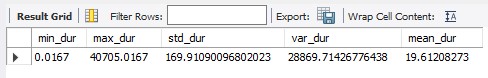
SELECT * FROM td_c WHERE duration < 0;
The result is:

My hypothesis proved accurate. The start date has a bigger value than the end date, and the data appeared to be swapped. Now, to resolve this issue, I only need to swap the data using the following SQL script:
UPDATE cyclistic.td_all
SET started_at = (@tmpDate:=started_at),
    started_at = ended_at,
    ended_at = @tmpDate
WHERE timestampdiff(second, started_at, ended_at) < 0;

/* result: 108 rows affected*/
EXPLANATION: In the SET statement, the first started_at was a dictionary to make a temporary date values consist of the raw start date data. Then, in the second started_at, I replace the start date to end date. Finally, the end date was replaced by the raw start date data using the temporary date values defined before.
To verify that there are no remaining negative durations, I used the same SQL script to examine the data with negative duration. If the result is 0, the problem has been resolved. After that, I re-executed the SQL script for the summary table to observe changes in data distribution; the outcome was:
/* First create a table by copying table schema as same as the td_all table */
CREATE TABLE td_cl LIKE td_all;

/* Add new columns and specifiy its data type by altering the new table */
ALTER TABLE cyclistic.td_cl
    ADD day_name text,
    ADD month_name text,
    ADD duration float;

/* Insert data into new table using SELECT statement,
duration is in MINUTE*/
INSERT INTO cyclistic.td_cl
			SELECT
				*,
				dayname(started_at) as day_name,
                monthname(started_at) as month_name,
				timestampdiff(second, started_at, ended_at)/60 as duration
			FROM
				cyclistic.td_all
			WHERE
				timestampdiff(second, started_at, ended_at) <> 0 AND
                start_station_name <> end_station_name AND
				(start_lat <> end_lat AND start_lng <> end_lng);
            /* First filter filtered out 0 second data
            and second filter filtered out the false ride
            such as error, redocking bike or cancel ride. */
I used Power BI as the analysis tool and MySQL Connector/NET to connect the database to the MySQL local server. I added day_num, month_num, and year_num columns within Power BI to provide day_name and month_name columns with date hierarchy context. For this, I used the following DAX script:
// Day of the week order numbers //
day_num = WEEKDAY('cyclistic td_cl'[started_at],1)

// Month order numbers //
month_num = MONTH('cyclistic td_cl'[started_at])

// Year order numbers //
year_num = YEAR('cyclistic td_cl'[started_at])
EXPLANATION: The value 1 in the WEEKDAY() function implies that Sunday, the first day of the week, equals 1 (the default value for the first day of the week is 0). The MONTH() function starts counting January as 1 by default. And YEAR() function will return the oldest year as 1, so 2021 will be 1 and 2022 will be 2.
Afterward, I wanted to create condensed day_name and month_name columns by taking the initial three letters, using this DAX script:
// Use this for month name too //
day_name_short = LEFT('cyclistic td_cl'[day_name], 3)
For the last, I made a distance column by computing the start and end station latitude and longitude using the Haversine formula so we would have a distance data in Kilometer. The DAX script is:
distance =
    var R = 6371
    var rad_factor = 0.0174533
    var lat1 = (90 - 'cyclistic td_cl'[start_lat]) * rad_factor
    var lat2 = (90 - 'cyclistic td_cl'[end_lat]) * rad_factor
    var lng_diff = ('cyclistic td_cl'[start_lng] - 'cyclistic td_cl'[end_lng]) * rad_factor
    var results = R * ACOS((COS(lat1)*COS(lat2)) + (SIN(lat1)*SIN(lat2)*COS(lng_diff)))
return results
By now, table is ready for further analysis.
In this analysis I want to collect the basic information about riders, bikes, and riders' activities.

The member plot has a higher center of distribution than the casual plot, with a median of 8,500. Q1 was approximately 4,400 while Q3 was 12,200.
The 200-point difference was seen as a normal distribution. In contrast to the casual plot, the lower whisker in the member plot was longer than the upper, indicating that there was a higher variance of values below the Q1 to minimum — which is likely to be inaccurate considering that the 50 percent value of the data was so nearly to the maximum. In addition, it was discovered that there were potential outliers above the upper and below the lower whiskers, although the value appeared to be more condensed compared to the casual plot. With an IQR of 7,500 for the casual plot and 7,800 for the member plot, the data in the member plot was slightly more dispersed than in the casual plot.
Next, the image below shows the distribution of total duration for both riders per day.

Member plot was normally distributed represented as shorter box lengths and equal whisker lengths. In contrast, the casual box plot was longer than the member, indicating that the data were more distributed. Box position was close to the minimum, indicating that values from Q3 to maximum were inaccurate, while median was close to Q1, indicating that the data distribution were positively skewed. Potential outliers were observed in both plots, but the proportion of potential outliers in the casual plot was significantly higher than in the member plot, indicating a large variation in values for the casual data.
The image below shows the distribution of total distance in both riders per day.
The distribution of the member plot was normal, whereas the distribution of the casual plot was positively skewed. IQRs for both plots were presumably equal. Longer upper whisker in the casual plot indicates a large variance in the data, indicating that the values above the Q3 to maximum are most likely inaccurate.
SUMMARIES:
Our service was frequently used by member riders. It was concluded that the member riders had a normal distribution for the total rides, total duration, and total distance. Casual riders used our service irregularly. Eventhough, it appeared that they contributed to the greater quantity of length and distance, as indicated by a longer upper whisker and a right-skewed box (positively skewed distribution). Additionally, it was observed on possible outliers above the upper whisker, which values could reach extremely high. These statements will be tested in further analysis.
This section analyzed general data to obtain information such as our service's performance, who used the most, which products riders preferred, and patterns. Initially, the figure below shows the total number of monthly rides per year.
The chart is distinct and the pattern is immediately identifiable. The number of riders decreased from October 2021 to January 2022 (-83% from October 2022), then increased from February 2022 to July 2022 (+86.25 % from February 2022). What makes it distinctive is that it began lowering again in August 2022 and is expected to keep falling until January 2023. I can conclude that there is a six-month window during which people will or will not use our service. There may be seasonal or other situations preventing consumers from using our services.
The next question is who uses our services the most?
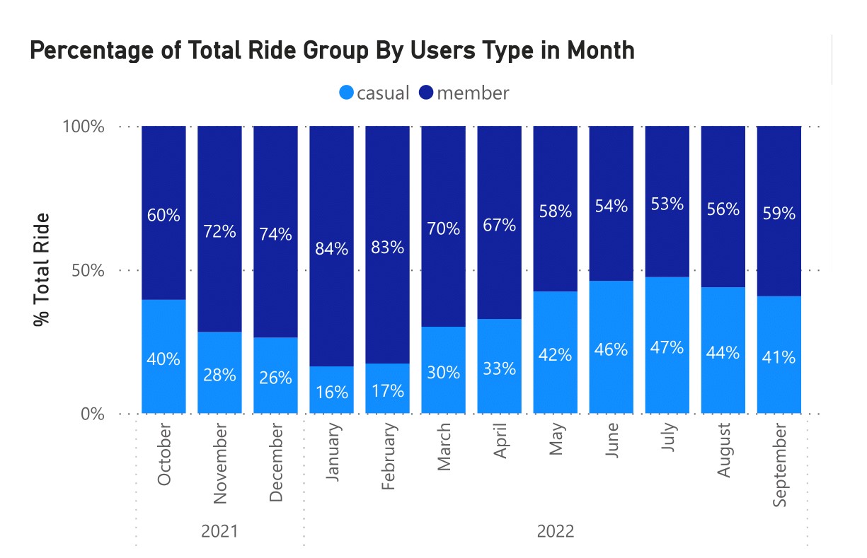
The image above shows that our services were largely used by our member riders. Even though there was a small difference for casual riders in July 2022, as previously stated, we can conclude that member riders used our service on a regular basis, with more than 50 percent coverage per month.
Now, what bikes used the most?

Classic and electric bikes were the most popular, whereas docked bikes were used less than 5% of the time per month. Who then uses these bikes?

It is apparent that only member riders used classic and electric bikes, whilst only casual riders used docked bikes. Even though the annual total usage rate of docked bikes was only 3.9%, it was still interesting to consider. member riders may make up the majority of monthly usage, but how long did they ride the bike each month?

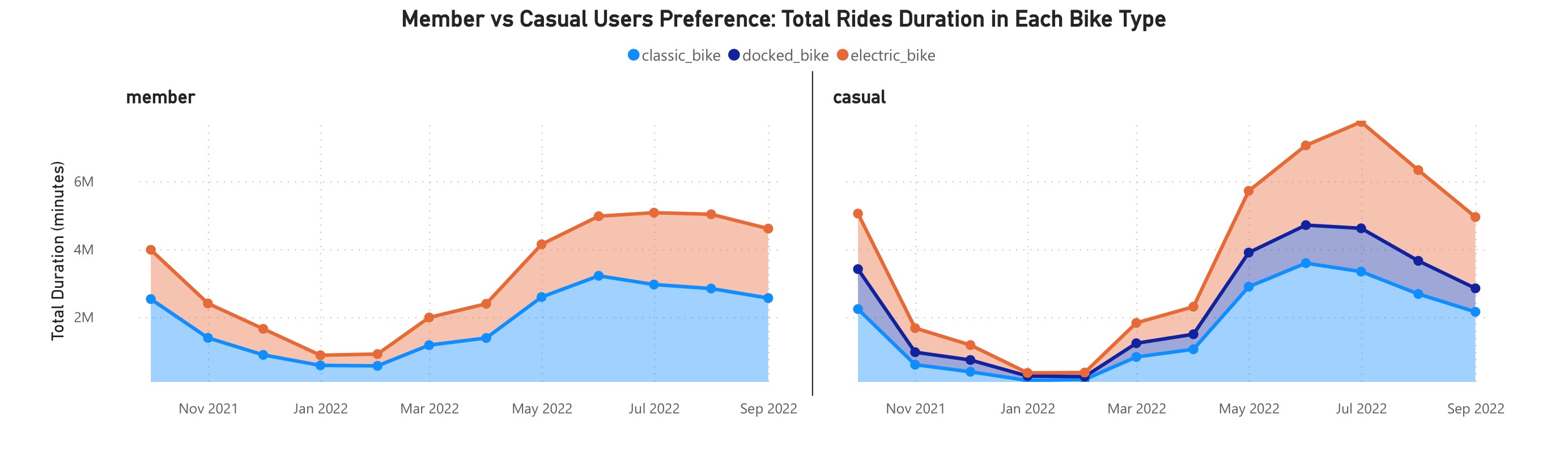
On the stacked area chart above, total duration for member riders was greater than for casual riders from November 2021 to February 2022, then nearly equaled in March to April 2022. After that, casual riders had a greater usage duration than member riders. The peak was in July 2022, with a total of 7.7 million minutes for 337,905 casual riders and 5 million minutes for 374,775 member riders. Which means that average usage for casual and member riders in July was 22.8 and 13.3 minutes per user, respectively. What about the bikes? Which bikes had a longer duration usage?

It turns out that classic bikes always dominate the usage duration. It went slightly different with the electric bike from November 2021 to April 2022. In July 2022, docked bike duration usage covered 20% of classic bike duration. Also, average duration usage in the same month was 51.76 minutes per usage for docked bikes, compared to classic and electric bikes that only had average usage of 18.15 and 15.40 minutes per usage, respectively. Considering the docked bike riders were only casual riders, it could be concluded that casual riders use our service for a longer duration than member riders.
SUMMARIES:
There were 6-month pattern where our riders use the most and the least our services. Member riders used our service regularly in higher frequency than the casual riders. Meanwhile, the casual riders used our service longer than member riders. Member riders only used classic and electric bikes while the casual riders used all three type of bikes Eventhough the docked bike is the least interested, but it was used for the longer duration than the others.
In this analysis, I compared member riders and casual riders data about their preferences and behaviors in using our service. Firstly, I wanted to know what bikes they used the most, so I continued previous analysis by specifying it onto two different groups.

In the stacked area chart above, member riders used classic bike more often than electric bike. Meanwhile, casual riders used electric bike more often than the classic bike. Which one used longer in duration?
The chart above told that classic bike was longer used than the electric bike for member riders. It showed the linear relationship between the total rides and total duration for member riders. The results showed to be different for the casual riders. Classic bike was longer used than the electric bike — which seen from January 2022 — even they used electric bike more. Now, what was the average duration?

The results was surprising, member riders average duration usage were stable in 12 minutes for each bike per month. It showed completely different result for the casual riders; docked bike used irregularly with the biggest average duration usage (more than 40 minutes per month), but the they used classic and electric bikes regularly with average duration of 21 and 15 minutes, respectively. These results confirmed previous analysis hypothesis that member riders used our service more often and regular than the casual riders, while the casual riders used longer than member riders.
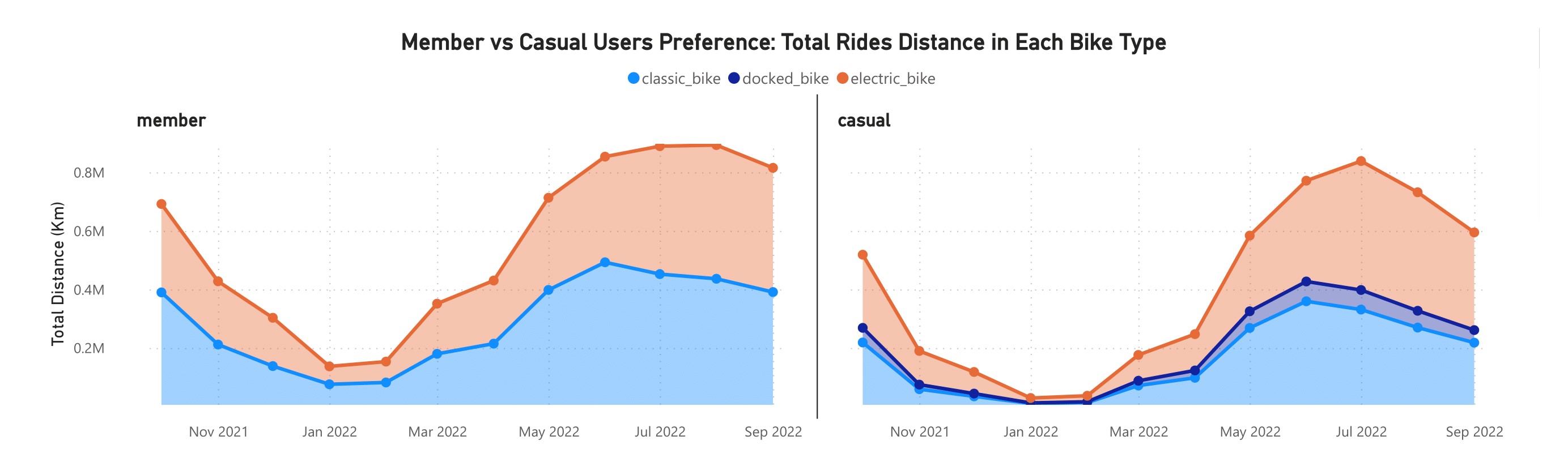
As shown in the chart above, the monthly total distance follows a similar pattern as the monthly total duration. There was a slightly difference in the total distance traveled by member riders using electric and classic bikes; sometimes they traveled a longer distance using classic bikes, and sometimes they traveled a longer distance using electric bikes. While casual riders primarily rode electric bikes further than classic and docked bikes, during a specific time period (such as May to June 2022), classic bikes were used further than electric bikes. It must be determined whether there is a correlation between duration and distance.
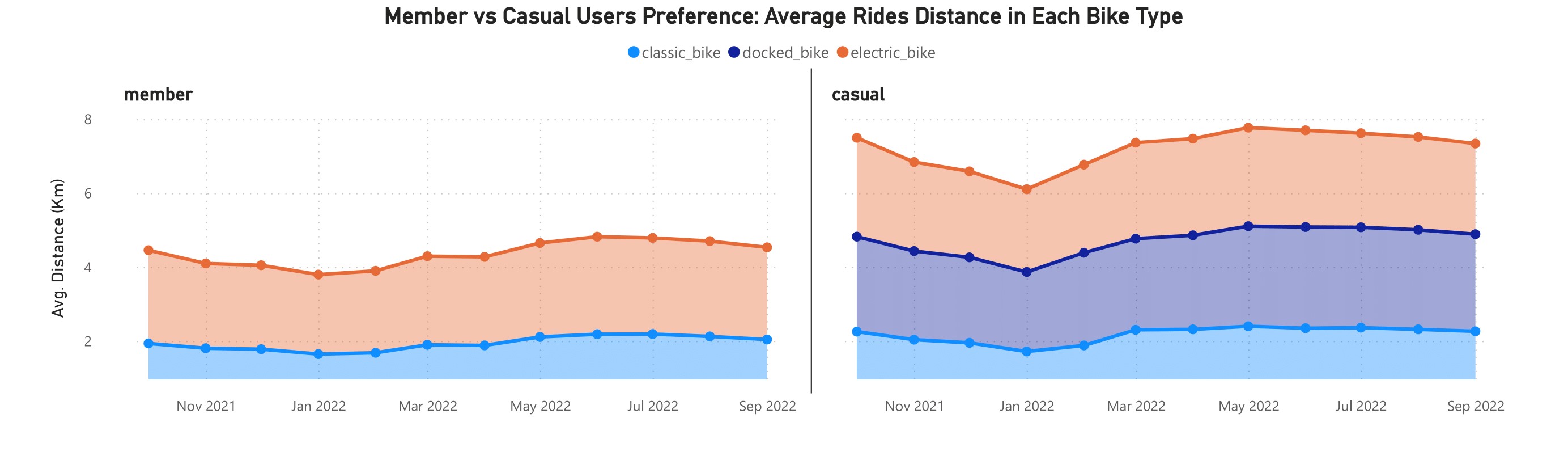
Even though the average duration was the same (12 minutes), member riders rode electric bikes farther than classic bikes; 2.15 to 2.64 kilometers versus 1.65 to 2.19 kilometers. Meanwhile, the average distance traveled by casual riders is likely to be comparable for all three types of bikes: 2.24-2.67 km for electric bikes, 1.72-2.4 km for classic bikes, and 2.15-2.74 km for docked bikes. Despite the irregular use of docked bike, the average distance was considered stable within the previously mentioned range. In January 2022, its average duration was 40 minutes, but its average distance was only 2.15 kilometers.

This scatter plot examined the linear correlation between duration on the x-axis and distance on the y-axis using Pearson's correlation coefficient (r value). Because it generated a significant discrepancy with other data, duration values above 1,440 minutes (24 hours) were filtered out. As shown by the scatter plot, the correlation between the two sets of data was not linear; a negative line may indicate a negative correlation, but the r values do not support this interpretation. Since the data did not follow a linear distribution and the trend line indicated a negative correlation, the r value for member plot (r = 0.41) may be a false positive.
The r value for the casual riders indicated that there may be no correlation (r = -0.02). Using a combination of member and casual data, I also ran Pearson's correlation test, which revealed a very weak correlation (r = 0.17). This may indicate that ride duration is not directly related to the distance traveled by riders, or that the correlation is non-linear.
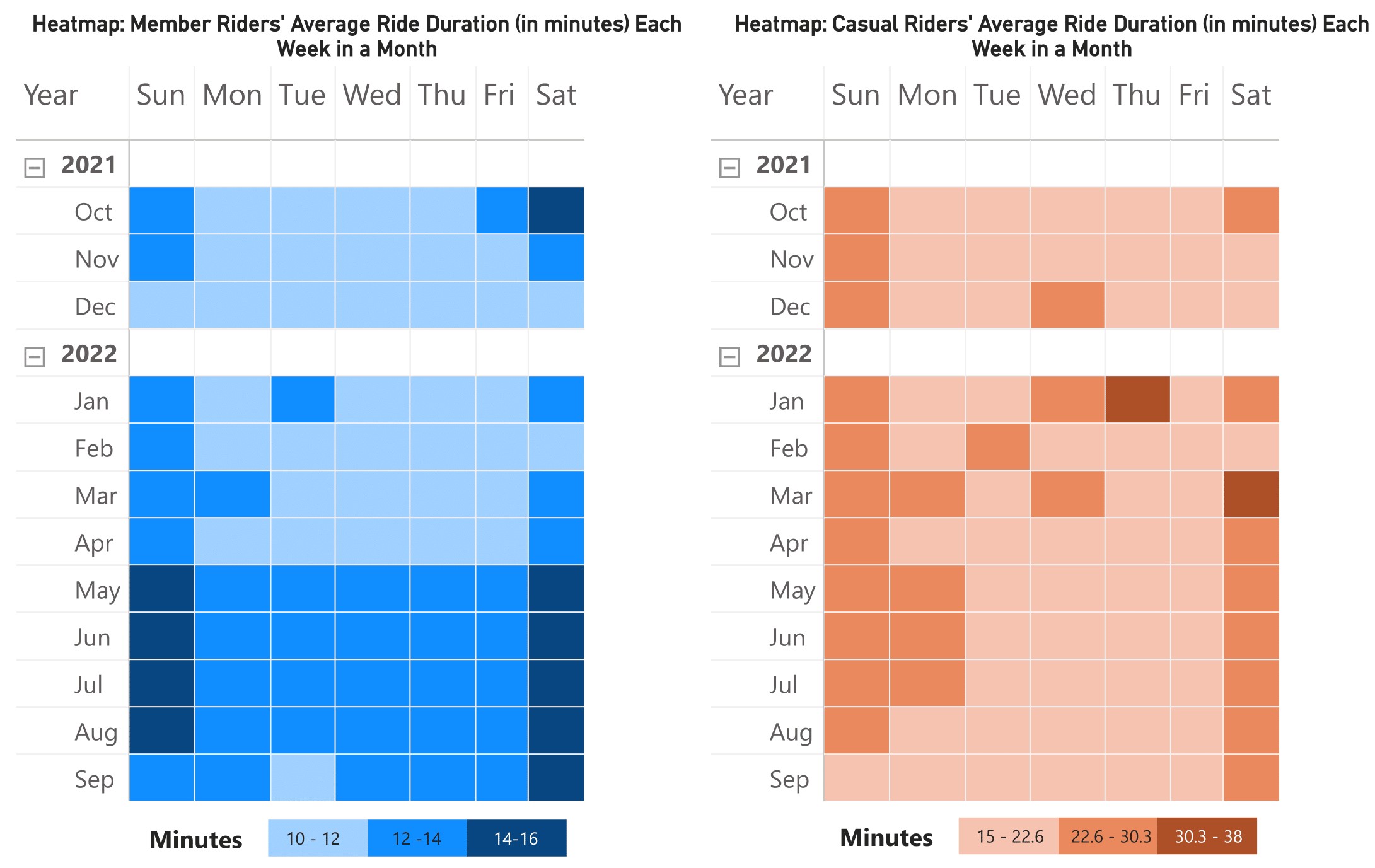
The heatmap above depicts the average riding duration per day in a month. Both riders rode for a longer duration on weekends and regularly in a lower range during the weekdays. Unlike casual riders, member riders average duration increased from May to September 2022, both on weekdays and weekends. This finding might cause confusion because, according to the prior analysis, the total and average ride duration for casual riders increased during the same time period, but the heatmap doesn't reflect the same result. This can be explained if we go back to the total duration distribution test in the 4.2.1 Data Distribution section .
As discussed previously, the daily total duration data for casual riders was greatly dispersed. It means that there would be a day with the longest duration in one week and the shortest duration in the other weeks. When it comes to the calculation, the result will be in the relatively same range and will be less sensitive to recognizing changes. This may explain why there were no changes depicted in the heatmap. Meanwhile, member riders had normally distributed daily total duration data. So, the results of the calculation will be more sensitive to changes. This is why the increasing average duration could be depicted in the heatmap.

The map shown above highlights which stations were the most popular as the starting points for member riders. This analysis is required to reveal the activity of riders. It may provide a information as to where riders lived or worked, such as if the station was located near a residence, business area, school area, or tourism area. I did not do the analysis for the end station because the end station could be the new starting station (for riders who did a round trip). Thus, I consider it is adequate to represent both the start and end stations. In the table below, I have compiled a list of the top 10 stations as well as the names of the nearby areas (list are sorted alphabetically).
| # | Station | Nearby Areas |
|---|---|---|
| 1. | Clark St. & Elm St. | The Elm at Clark (apartments), Elm Street Plaza, Mark Twan Hotel, Clark & Elm bus station |
| 2. | Clinton St. & Madison St. | West Loop Gate, Chicago OTC train station, Clinton & Madison Bus stations, Presidential Towers, AT&T Canal Central Office, Ogilvie Transportation Center, Zurich Insurance Co. |
| 3. | Clinton St. & Washington St. | |
| 4. | Ellis Ave. & 60th St. | University of Chicago, Burton-Judson Courts, Edelston Center, Fiske Elementary School |
| 5. | Kingsbury St. & Kinzi St. | River North Point, Hubbard Place, Fulton River District, LuxeHome |
| 6. | Loomis St. & Lexington St. | Arrigo Park, Little Italy, Public Schools Jackson Andrew, Garibaldi Square |
| 7. | University Ave. & 57th St. | University of Chicago |
| 8. | Wells St. & Concord Ln. | American Towers (condominium houses) |
| 9. | Wells St. & Elm St. | Old Town Park, Atrium Village, LaSalle Court (apartments), LaSalle Street Church |
| 10. | Wells St. & Huron St. | Flair Tower, Seven, Marlowe (apartments) |
As seen in the table above, we can assume that member riders range in age from youth to adults. Two stations, including University Ave. & 57th St. and Ellis Ave. & 60th St., are in the University of Chicago area. I believed riders in this area to be college students, professors, and other employees. With this information, we can also hypothesize that riding activities are limited to the campus region.
The stations at Clark St. & Elm St., Wells St. & Concord Ln., Wells St. & Elm St., and Wells St. & Huron St. are close to the apartments and condominiums. It is assumed that the majority of riders in these locations are adults, whether they are married or not. Riders that ride at stations near the business or office areas such as Clinton St. & Madison St., Clinton St. & Washington St., and Ellis Ave. & 60th St. are likely adults who worked in the government or private sectors. Furthermore, all of those riders may use our service on a regular basis for their daily transportation, considering the proximity of the station to their residence and workplace.
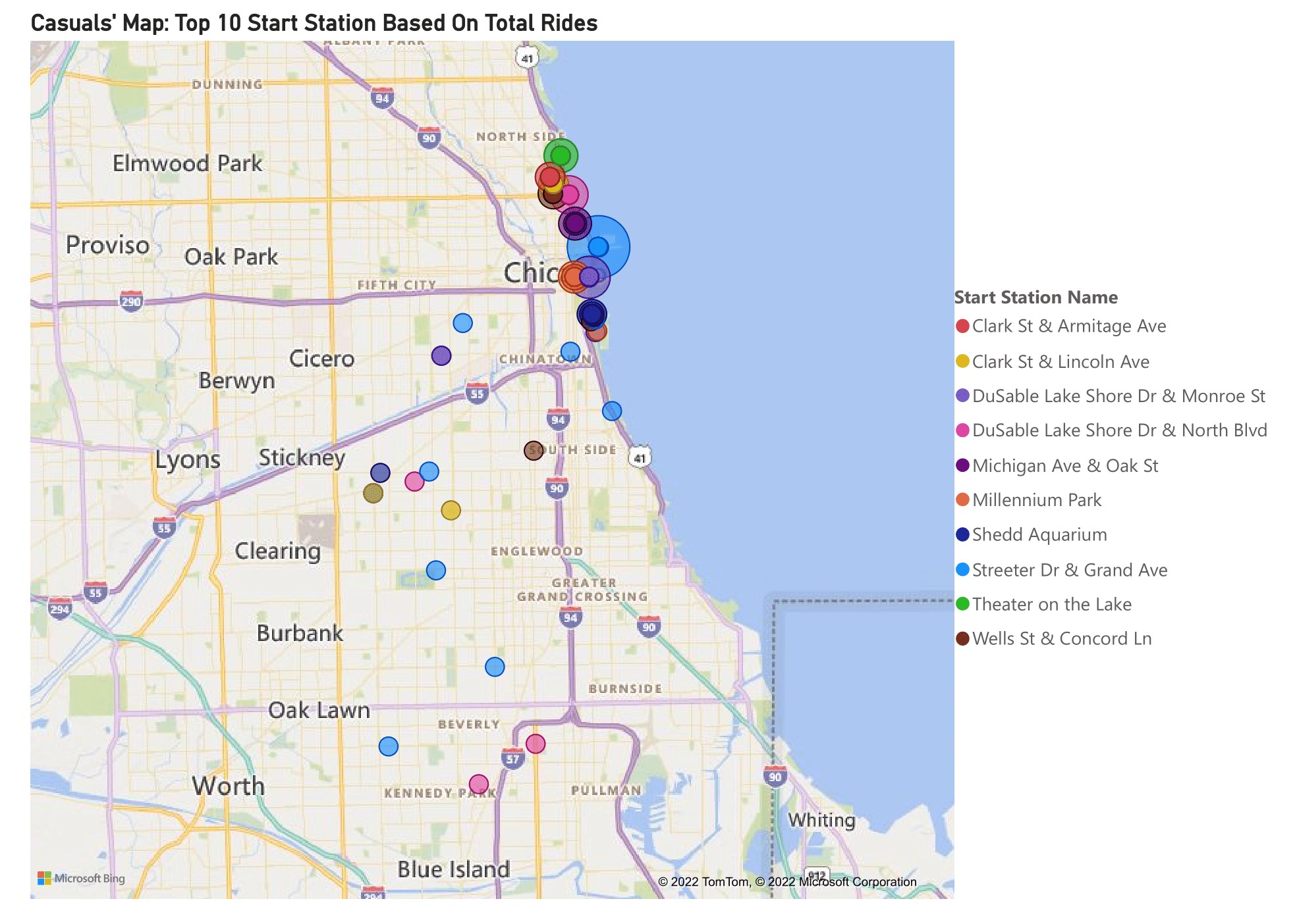
Visually, the result for casual riders was completely different. They used stations near Lake Michigan and DuSable Lake Shore Drive. To see more detail information, I created a list of the stations (sorted alphabetically) and their nearby areas in the table below.
| # | Station | Nearby Areas |
|---|---|---|
| 1. | Clark St. & Armitage Ave. | Lincoln Park Tower (apartments), Lincoln Park Zoo Administration Building, Armitage & Clark Bus Stations |
| 2. | Clark St. & Lincoln Ave. | Hemingway House (condominiums), Clark & Lincoln Bus Station, Lincoln Park Zoo |
| 3. | DuSable Lake Shore Dr. & Monroe St. | Chicago Yacht Club, Sailing Lake Michigan |
| 4. | DuSable Lake Shore Dr. & North Blvd. | 1550 North Lake Shore Drive (apartments), Lincoln Park |
| 5. | Michigan Ave. & Oak St. | 100 N Lake Shore Park, The Magnificent Mile (business, shopping, and hotel area) |
| 6. | Millennium Park | Millennium Park, Michigan Avenue (business and historic area), Michigan & Monroe bus station |
| 7. | Shedd Aquarium | Shedd Aquarium, Field Museum, The Great Ivy Lawn Park, Lakefront Trail (tourism area) |
| 8. | Streeter Dr. & Grand Ave. | Lake Point Tower (apartments), Jane Addams Memorial Park, Grand & Streeter Bus Station, Ohio Street Beach |
| 9. | Theater on the Lake | Theater on the Lake, The Lakefront Restaurant, Lakefront Trail-Fullerton, Fullerton Beach (tourism area and restaurant) |
| 10. | Wells St. & Concord Ln. | American Towers (condominiums) |
Even though there are stations close to apartments and condominiums, the majority of these locations are in areas close to tourist destinations. Except for Wells St. & Concord Ln. station, it is located more in the center of the city. Stations like Clark St. & Armitage Ave., Clark St. & Lincoln Ave., and DuSable Lake Shore Dr. located near the Lincoln Park area. Assuming that the majority of casual riders are tourists, Lincoln Park may be at the top of their minds as a tourist destination.
In addition, stations such as Millennium Park, Shedd Aquarium, and Theater on the Lake are located close to the tourist destination. Offering a special deal by combining tourism and our service will be a great potential strategy to attract casual riders to join as members. Other stations like Michigan Ave. & Oak St. are placed near the business district, which offers restaurants, dining, shopping, hotels, and historical places (e.g., museums). We need more information about what they need to become members.
SUMMARIES:
Members' average ride duration was equally 12 minutes for classic and electric bikes, or 24 minutes per month. Casuals' average ride duration was 21 minutes for classic bikes, 15 minutes for electric bikes, and up to 40 minutes for docked bikes. Members ride electric bikes farther than classic bikes, even though the average duration is the same. Casuals ride electric bikes farther than classic bikes, which are quite comparable to docked bikes.
There is no linear correlation between duration and distance for both riders.
Riders' activity was higher on weekends than on weekdays. There was an increase in activity for member riders from May to August 2022, both on weekdays and weekends.
There appeared to be a range of ages and professions among the members, from youth to adults and from students to professionals. It is assumed that members use our service as their daily transportation, considering the proximity to their residence, school, and workplace.
Considering how close they were to tourist areas, the majority of the casual riders seemed to be tourists, both local and international.
| Case Study Roadmap - Analyze |
|---|
Guiding Questions:
|
Key Tasks:
|
| Case Study Roadmap - Share |
|---|
Guiding Questions:
|
Key Tasks:
|
| Case Study Roadmap - Act |
|---|
Guiding Questions:
|
Key Tasks:
|